Research Design 2: Event Studies and Difference-in-Difference

Stijn Masschelein

── Attaching core tidyverse packages ──────────────────────── tidyverse 2.0.0 ──
✔ dplyr     1.1.4     ✔ readr     2.1.5
✔ forcats   1.0.0     ✔ stringr   1.5.1
✔ ggplot2   4.0.1     ✔ tibble    3.2.1
✔ lubridate 1.9.4     ✔ tidyr     1.3.1
✔ purrr     1.2.0     
── Conflicts ────────────────────────────────────────── tidyverse_conflicts() ──
✖ dplyr::filter() masks stats::filter()
✖ dplyr::lag()    masks stats::lag()
ℹ Use the conflicted package (<http://conflicted.r-lib.org/>) to force all conflicts to become errors

Attaching package: 'cowplot'


The following object is masked from 'package:lubridate':

    stamp


here() starts at /Users/stijnmasschelein/Dropbox/github/site


Attaching package: 'kableExtra'


The following object is masked from 'package:dplyr':

    group_rows

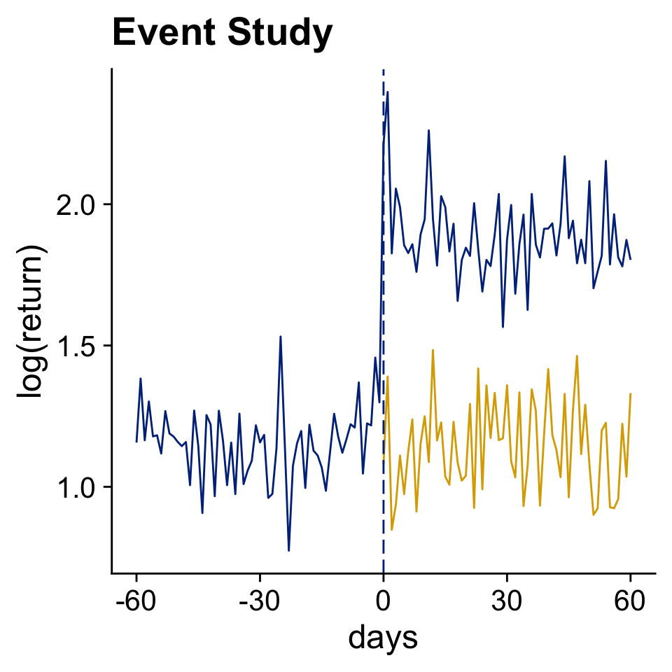
Event Studies

A basic before - after comparison

Chapter 17 Event Studies in Huntington-Klein (2021)

Where Time could be standing in for a lot of other annoying things that might happen.

Use Data Before The Event to Infer The Counterfactual Outcome (in Yellow)

We do not observe the yellow/gold returns. We have to estimate them or convince the reader that there are no trends to be expected for theoretical/institutional reasons. I will not go into the details of the estimation here but I will in week 7.

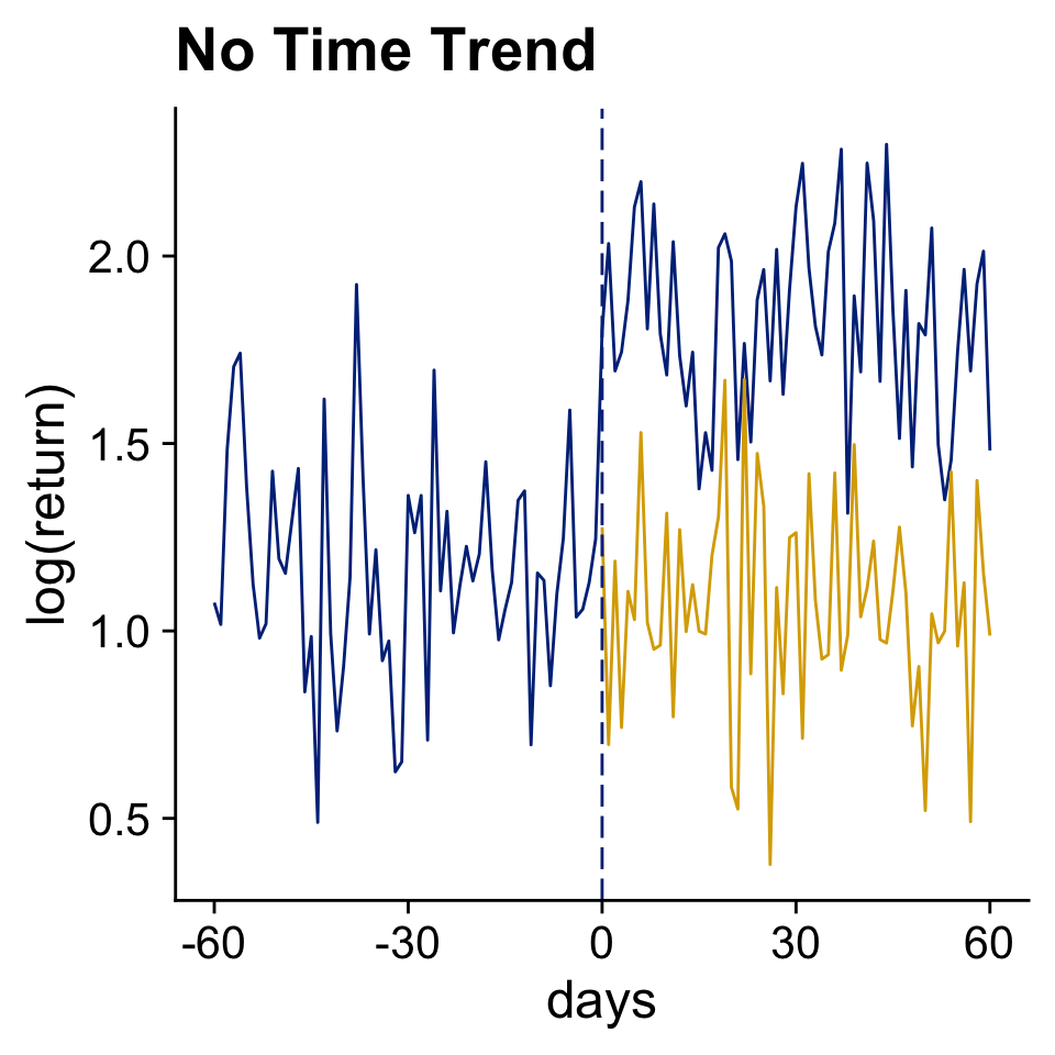
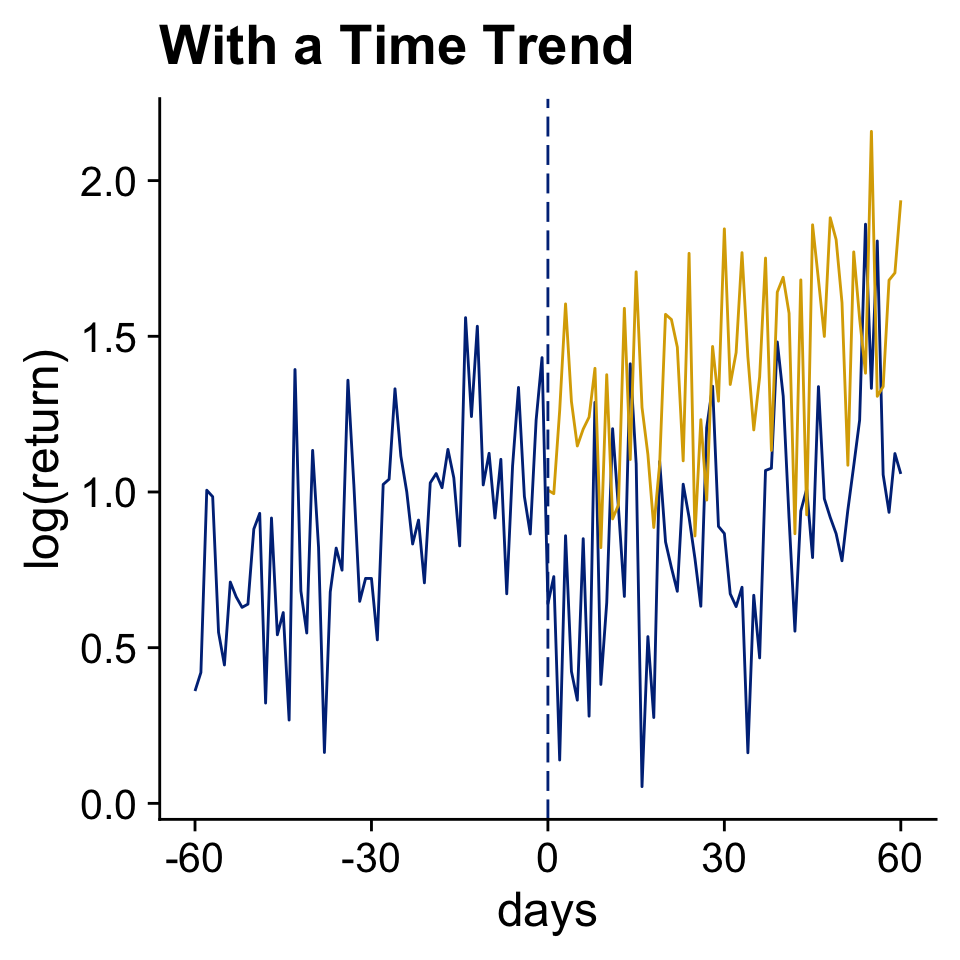
Front-running, information leaking, and anticipation are all annoying.

Go also back to Assignment 2 where we modeled the same problem when investors anticipate a donation.

To gauge demand from buyers and potentially gin up interest from sellers, bankers send out lists of shares with upcoming lockup expirations, according to market participants. (Money Stuff, Matt Levine)

Sometimes, bankers also engage in hypothetical conversations with buyers before they have a mandate. Asking prospective buyers whether they might be interested in certain stocks is one thing. But if there are indeed plans afoot for block sales, such conversations, even phrased hypothetically, can tip off savvy money managers. (Money Stuff, Matt Levine)

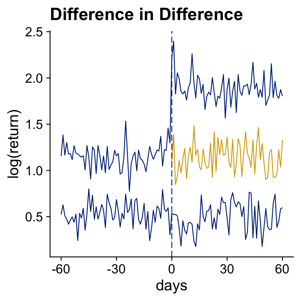
Difference-in-Difference

What if we had an additional control group to estimate the counterfactual?

A Simulated Cheap Talk Example: Voluntary Disclosure in Time 2

N <- 500
T <- 2
time_effect <- c(3.5, 0)
rd_did_firm <- tibble(
  firm = 1:N,
  performance = runif(N, 1, 10),
  firm_effect = rnorm(N, 0, 2) + ifelse(performance < 3, 3, 0)
)
rd_did_panel <- tibble(
  firm = rep(1:N, each = T),
  time = rep(1:T, times = N)) %>%
  left_join(rd_did_firm, by = "firm") %>%
  mutate(
    report = ifelse(time == 2, ifelse(performance > 3, 1, 0), 0),
    noise = rnorm(N*T, 0, 3),
    profit_report = 6.5 + time_effect[time] + firm_effect + noise,
    profit_no_report = 1.5 + time_effect[time] + firm_effect + noise,
    actual_profit = ifelse(report == 1, profit_report, profit_no_report))

The idea is that we have firms who perform well (performance > 3) and firms that perform bad (performance < 3). The firms that perform well will voluntarily disclose a report in time 2. We can see the effect as the difference between time 1 and time 2 for disclosers and non-disclosers.

Important: the cost of misreporting is not in calculated in the profit. The reasoning would be that this might be a litigation cost that would only emerge later on.

The Causal Effects in Our Simulation

rd_did_panel %>%
  mutate(causal_effect = profit_report - profit_no_report) %>%
  group_by(time, report2 = performance > 3) %>%
  summarise(profit_report = mean(profit_report),
            profit_no_report = mean(profit_no_report),
            causal_effect = mean(causal_effect)) %>%
  kable(digits = 1)

`summarise()` has grouped output by 'time'. You can override using the
`.groups` argument.

time	report2	profit_report	profit_no_report	causal_effect
1	FALSE	12.9	7.9	5
1	TRUE	10.0	5.0	5
2	FALSE	9.2	4.2	5
2	TRUE	6.4	1.4	5

A Summary of The Actual Profits

rd_did_panel %>%
  group_by(time, report2 = performance > 3) %>%
  summarise(actual_profit = mean(actual_profit)) %>%
  pivot_wider(names_from = time, values_from = actual_profit) %>%
  kable(digits = 1)

`summarise()` has grouped output by 'time'. You can override using the
`.groups` argument.

report2	1	2
FALSE	7.9	4.2
TRUE	5.0	6.4

Regressions

did_lm <- feols(actual_profit ~ report, data = rd_did_panel)
did_sub <- feols(actual_profit ~ report, data = filter(rd_did_panel, time == 2))
did_fixed <- feols(actual_profit ~ report | firm, data = rd_did_panel)
did_did <- feols(actual_profit ~ report | firm + time, data = rd_did_panel)
msummary(list(simple = did_lm, "time 2" = did_sub, "firm FE" = did_fixed, "two-way FE" = did_did),
         gof_omit = gof_omit, stars = stars)

	simple	time 2	firm FE	two-way FE
* p < 0.1, ** p < 0.05, *** p < 0.01
(Intercept)	5.338***	4.193***
	(0.153)	(0.363)
report	1.029***	2.174***	1.405***	5.142***
	(0.243)	(0.407)	(0.237)	(0.488)
Num.Obs.	1000	500	1000	1000
R2	0.018	0.054	0.612	0.662
R2 Within			0.066	0.183
RMSE	3.75	3.68	2.36	2.20
Std.Errors	IID	IID	IID	IID
FE: firm			X	X
FE: time				X

What if we have three periods?

Note

We assume that over time investors and regulators get better at detecting when firms exaggerate in their report.

• Time 1: Reports are not believable, nobody reports
• Time 2: The biggest exaggerations will be caught, only well performing firms will report and communicate that they are doing excellent.
• Time 3: More subtle exaggerations will be caught. The worst performers will not report at all, the moderate performers will report and say that they will do well, the good performers will report that they are doing excellent.

See the Appendix of the assignment for the derivation of the exact parameters.

Setup of three period simulation

N <- 1000
T <- 3
cutoff2 <- 3 # performance cutoff to report for time 1
cutoff3 <- c(4/3, 4 + 2/3) # performance cutoff to report for time 2
profit1 <- 5
profit2 <- c(1.5, 6.5) #Profits for time 2 depending on report
profit3 <- c(2/3, 3, 7 + 1/3) #Profits for time 2 depending on report
rd_did3_firm <- tibble(
  firm = 1:N,
  performance = runif(N, 0, 10),
  firm_effect = rnorm(N, 0, 2) + ifelse(performance < cutoff2, 3, 0)
)

Three period simulation

rd_did3_panel <- tibble(
  firm = rep(1:N, each = T),
  time = rep(1:T, times = N)) %>%
  left_join(rd_did3_firm, by = "firm") %>%
  mutate(
    # When will firms report?
    report = case_when(
      time == 1 ~ 0,
      time == 2 & performance < cutoff2 ~ 0,
      time == 3 & performance < cutoff3[1] ~ 0,
      TRUE ~ 1),
    noise = rnorm(T*N, 0, 5),
    profit_no_report = firm_effect + noise +
      case_when(
        time == 1 ~ profit1,
        time == 2 ~ profit2[1],
        time == 3 ~ profit3[1]
    ),
    profit_report = firm_effect + noise +
      case_when(
        time == 1 ~ profit1,
        time == 2 ~ profit2[2],
        time == 3 & performance < cutoff3[2] ~ profit3[2],
        TRUE ~ profit3[3]
      ),
    actual_profit = ifelse(report == 1, profit_report, profit_no_report)
  )

Overview of 4 groups of firms

1. Never reporters
2. Reporters in year 3
3. Reporters in year 2 and 3 (Medium)
4. Reporters in year 2 and 3 (High)

causal_effects <- rd_did3_panel %>%
  mutate(causal_effect = profit_report - profit_no_report,
         group = case_when(
           performance < cutoff3[1] ~ 1,
           performance < cutoff2 ~ 2,
           performance < cutoff3[2] ~ 3,
           TRUE ~ 4
         )) %>%
  group_by(time, group) %>%
  summarise(report = mean(report),
            N = n(),
            M_report = mean(profit_report),
            M_no_report = mean(profit_no_report),
            M_causal_effect = mean(causal_effect))

`summarise()` has grouped output by 'time'. You can override using the
`.groups` argument.

Overview of 4 groups of firms

time	group	report	N	M_report	M_no_report	M_causal_effect
1	1	0	157	8.6	8.6	0.0
1	2	0	157	8.3	8.3	0.0
1	3	0	188	5.0	5.0	0.0
1	4	0	498	5.1	5.1	0.0
2	1	0	157	9.6	4.6	5.0
2	2	0	157	9.6	4.6	5.0
2	3	1	188	6.9	1.9	5.0
2	4	1	498	6.8	1.8	5.0
3	1	0	157	5.9	3.5	2.3
3	2	1	157	5.8	3.5	2.3
3	3	1	188	2.6	0.3	2.3
3	4	1	498	7.6	0.9	6.7

Two-way Fixed Effects

twoway12 <- feols(actual_profit ~ report | firm + time,
                  data = filter(rd_did3_panel, time != 3))
twoway13 <- feols(actual_profit ~ report | firm + time,
                  data = filter(rd_did3_panel, time != 2))
twoway123 <- feols(actual_profit ~ report | firm + time,
                  data = rd_did3_panel)

Separate 2 by 2 effects are larger than the total sample effect

msummary(list("time 1 and 2" = twoway12, "time 1 and 3" = twoway13,
              "time 1, 2 and 3" = twoway123), gof_omit = gof_omit,
         stars = c("*" = .1, "**" = .05, "***" = .01))

	time 1 and 2	time 1 and 3	time 1, 2 and 3
* p < 0.1, ** p < 0.05, *** p < 0.01
report	5.666***	5.565***	4.616***
	(0.475)	(0.634)	(0.404)
Num.Obs.	2000	2000	3000
R2	0.608	0.601	0.456
R2 Within	0.125	0.072	0.061
RMSE	3.48	3.64	4.17
Std.Errors	IID	IID	IID
FE: firm	X	X	X
FE: time	X	X	X

This is not what I would expect. Why would the full sample lead to a smaller effect than all the subsamples?

Baker, Larcker, and Wang (2022)

The paper is forthcoming in JFE but available on ssrn

Problem Statement

Finally, when research settings combine staggered timing of treatment effects and treatment effect heterogeneity across firms or over time, staggered DiD estimates are likely to be biased. In fact, these estimates can produce the wrong sign altogether compared to the true average treatment effects.

Solution

While the literature has not settled on a standard, the proposed solutions all deal with the biases arising from the “bad comparisons” problem inherent in TWFE DiD regressions by modifying the set of effective comparison units in the treatment effect estimation process. For example, each alternative estimator ensures that firms receiving treatment are not compared to those that previously received it.

Again, the solution to all our problems is to make sure that we make the right comparison.

Simulation Setup - The True Average Treatment Effect of Three Groups

It’s clear that the average treatment effect should be positive. It’s positive for every group.

The Estimated Effect by Twoway Fixed Effects of 500 Simulations

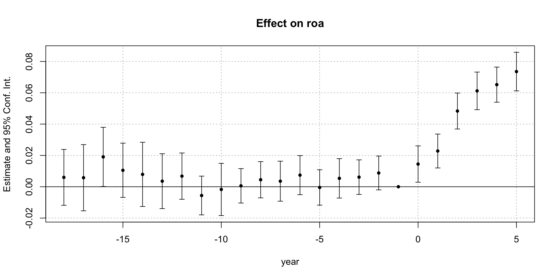
The Sun and Abraham (2021) Solution - Restrict The Sample

The Estimated Effect with the Sun and Abraham Solution

Sun and Abraham in Practice

sa_new <- readRDS(here("data", "sa_new.RDS"))
sa_fe <- feols(roa ~ 1 + sunab(treatment_group, year) | firm + year,
               cluster = "state", data = sa_new)

NOTE: 261/0 fixed-effect singletons were removed (261 observations).

sa_fe_att <- summary(sa_fe, agg = "ATT")
sa_fe_group <- summary(sa_fe, agg = "cohort")

• treatment_group: first year of treatment
• year: calendar year

names(sa_fe$coefficients)

 [1] "year::-18:cohort::1998" "year::-17:cohort::1998" "year::-16:cohort::1998"
 [4] "year::-15:cohort::1998" "year::-14:cohort::1998" "year::-13:cohort::1998"
 [7] "year::-12:cohort::1998" "year::-11:cohort::1998" "year::-10:cohort::1998"
[10] "year::-9:cohort::1989"  "year::-9:cohort::1998"  "year::-8:cohort::1989" 
[13] "year::-8:cohort::1998"  "year::-7:cohort::1989"  "year::-7:cohort::1998" 
[16] "year::-6:cohort::1989"  "year::-6:cohort::1998"  "year::-5:cohort::1989" 
[19] "year::-5:cohort::1998"  "year::-4:cohort::1989"  "year::-4:cohort::1998" 
[22] "year::-3:cohort::1989"  "year::-3:cohort::1998"  "year::-2:cohort::1989" 
[25] "year::-2:cohort::1998"  "year::0:cohort::1989"   "year::0:cohort::1998"  
[28] "year::1:cohort::1989"   "year::1:cohort::1998"   "year::2:cohort::1989"  
[31] "year::2:cohort::1998"   "year::3:cohort::1989"   "year::3:cohort::1998"  
[34] "year::4:cohort::1989"   "year::4:cohort::1998"   "year::5:cohort::1989"  
[37] "year::5:cohort::1998"  

Sun and Abraham - Relative Year

msummary(sa_fe, gof_omit = gof_omit, stars = stars, statistic = NULL,
         estimate = "{estimate} ({std.error}) {stars}", coef_omit = "-1")

	(1)
year = -9	0.014 (0.006) **
year = -8	0.004 (0.008)
year = -7	0.007 (0.006)
year = -6	0.008 (0.007)
year = -5	0.017 (0.006) ***
year = -4	0.008 (0.006)
year = -3	0.007 (0.006)
year = -2	0.004 (0.004)
year = 0	0.018 (0.006) ***
year = 1	0.028 (0.006) ***
year = 2	0.047 (0.006) ***
year = 3	0.061 (0.006) ***
year = 4	0.073 (0.006) ***
year = 5	0.080 (0.006) ***
Num.Obs.	111584
R2	0.724
R2 Within	0.006
RMSE	0.17
Std.Errors	by: state
FE: firm	X
FE: year	X

Sun and Abraham - Relative Year

iplot(sa_fe)

Sun and Abraham - ATT

msummary(sa_fe_att, gof_omit = gof_omit, stars = stars)

	(1)
* p < 0.1, ** p < 0.05, *** p < 0.01
ATT	0.051***
	(0.005)
Num.Obs.	111584
R2	0.724
R2 Within	0.006
RMSE	0.17
Std.Errors	by: state
FE: firm	X
FE: year	X

Sun and Abraham - Cohort Effects

msummary(sa_fe_group, gof_omit = gof_omit, stars = stars)

	(1)
* p < 0.1, ** p < 0.05, *** p < 0.01
cohort = 1989	0.055***
	(0.006)
cohort = 1998	0.047***
	(0.006)
Num.Obs.	111584
R2	0.724
R2 Within	0.006
RMSE	0.17
Std.Errors	by: state
FE: firm	X
FE: year	X

Take-away Lessons

Note

• Simulations are good!
• Everything is a regression (Ok, not really)
• Not all the data should go in the regression

When should you cluster standard errors?

Abadie et al. (2017)

Note

What is the level of the treatment variable? What is the comparison?

• Mixed race or same-sex race
• State legislation
• Country legislation
• Firm corporate governance changes

References

Abadie, Alberto, Susan Athey, Guido W. Imbens, and Jeffrey Wooldridge. 2017. “When Should You Adjust Standard Errors for Clustering?” Working {{Paper}}. Working Paper Series. National Bureau of Economic Research. https://doi.org/10.3386/w24003.

Baker, Andrew C., David F. Larcker, and Charles C. Y. Wang. 2022. “How Much Should We Trust Staggered Difference-in-Differences Estimates?” Journal of Financial Economics 144 (2): 370–95. https://doi.org/10.1016/j.jfineco.2022.01.004.

Huntington-Klein, Nick. 2021. The Effect: An Introduction to Research Design and Causality. First. Boca Raton: Chapman and Hall/CRC. https://doi.org/10.1201/9781003226055.

Sun, Liyang, and Sarah Abraham. 2021. “Estimating Dynamic Treatment Effects in Event Studies with Heterogeneous Treatment Effects.” Journal of Econometrics, Themed Issue: Treatment Effect 1, 225 (2): 175–99. https://doi.org/10.1016/j.jeconom.2020.09.006.