Quadratic and Cubic Terms in Linear Models.
In our weekly seminar, Robert Faff presented a paper with an OLS model with the quadratic and cubic term effects. The dependent variable in this model is the change in cash holdings (\(\Delta CH\)) by a company and the independent variable is the deviation of current cash holding from the optimal level (\(\Delta OPT\)). The paper argues that there are three different regimes of adjustment speed of cash holdings. Very high cash holdings will lead to the largest adjustment back to the optimal level, very low cash holdings will lead to a large but smaller adjustment towards the optimal level, the medium level of cash holdings leads to the smallest (or no) adjustment. This is the motivation to use a cubic model.
The relevant part of the OLS model is
\[ \Delta CH_i = \beta_0 + \beta_1 \Delta OPT_i + \beta_2 \Delta OPT_i^2 + \beta_3 \Delta OPT_i^3 + \epsilon_i \]
The results show that \(\beta_0 = -0.0038\), \(\beta_1=0.2633\), \(\beta_2=-0.0790\), and \(\beta_3=0.3827\). The problem is that those coefficients alone do not necessarily tells us anything about the three regimes and the speed of cash holding adjustment. Typically we are interested in the marginal effect of a variable. In this case the speed of adjustment which you can see as
\[ \frac{\partial \Delta CH}{\partial \Delta OPT} = \beta_1 + 2 \beta_2 \Delta OPT + 3\beta_3 \Delta OPT^2 \]
You can see that the speed of adjustment depends on three coefficients and the
value of \(\Delta OPT\). One way to represent the effect of \(\Delta OPT\) on
\(\Delta CH\) is to give the effect for different levels of \(\Delta OPT\) and that
is what the paper does. Another way of doing that is to make a plot. I quickly
show how you can do that in R.
First of all, I have to make a couple of assumptions because I don’t have the
full data. From the descriptive statistics, we know the meand (mopt) and
(sdopt) for \(\Delta OPT\). From those we can generate the distribution of
deviations. I tried two options: a normal distribution (opt_dev_norm) and a
t-distribution with 3 degrees of freedom (opt_dev_t). The latter will give
us larger outliers. Than we just calculate the cash holding change based on
the ’s above and the OLS specification. Finally, you can plot the relation
between change in cash holding and the deviation from the optimal level.
What struck me was that the three regimes are much more clear with the t-distribution than with the normal distribution for the deviations. In other words, it looks like the extreme cases are doing a lot of work to identify the regimes.
require(ggplot2)## Loading required package: ggplot2mopt = -0.0026
sdopt = 0.1488
opt_dev_norm = rnorm(1e4, mopt, sdopt)
opt_dev_t = rt(1e4, df = 3) * sqrt(sdopt^2/3) + mopt
round(quantile(opt_dev_norm, probs = c(0.75, 0.5, 0.25)), 2)## 75% 50% 25%
## 0.1 0.0 -0.1round(quantile(opt_dev_t, probs = c(0.75, 0.5, 0.25)), 2)## 75% 50% 25%
## 0.06 0.00 -0.07cash_change_norm = -0.0038 + 0.2633 * opt_dev_norm - 0.0790 * opt_dev_norm ^ 2 +
0.3827 * opt_dev_norm ^ 3
normplot = qplot(x = opt_dev_norm, y = cash_change_norm) +
ggtitle("Normal distributed deviations") +
theme_classic()
cash_change_t = -0.0038 + 0.2633 * opt_dev_t - 0.0790 * opt_dev_t ^ 2 +
0.3827 * opt_dev_t ^ 3
tplot = qplot(x = opt_dev_t, y = cash_change_t) +
ggtitle("T distributed deviations") +
theme_classic()
print(normplot)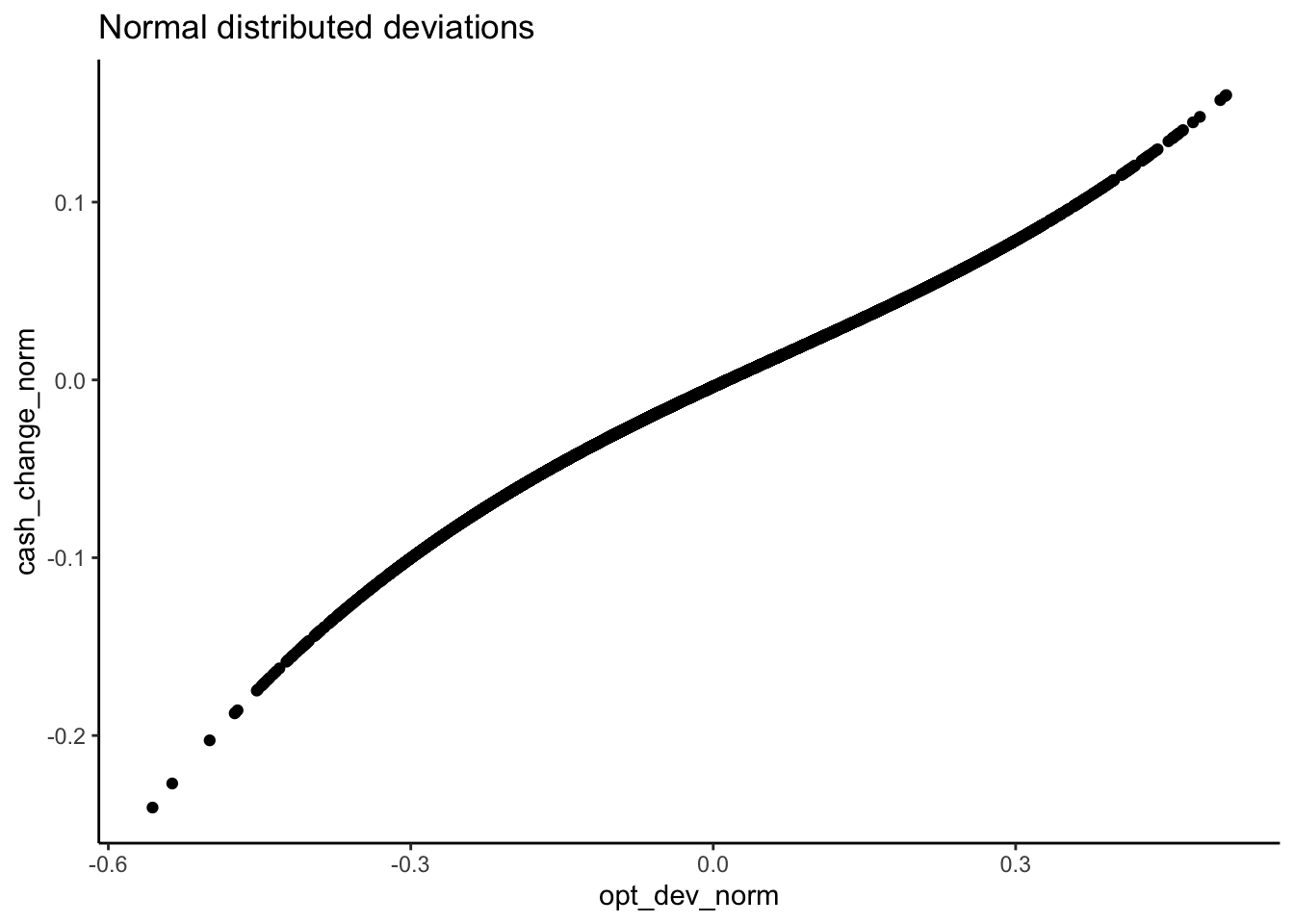
print(tplot)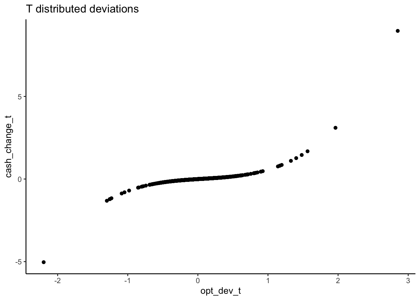
Stijn Masschelein
Senior Lecturer in Accounting and Finance - Fellow in Center of Data Business Analytics
I am a lecturer in accounting at the University of Western Australia. I am interested in the role of (management accounting) information in decision making and risk taking. My research investigate how verifiable and subjective information supports formal and informal contracts. My interest is easily piqued and as a result I am involved in a wide variety of projects such as field applications in target setting and cost of quality, lab experiments on negotiations, markets, and risk taking, survey research on integrity and quantitative field studies in the banking sector. I developed experience in a range of statistical methods such as meta-analysis, (Bayesian) multilevel models, and simulations.