Control Variables
Stijn Masschelein
Causal Graphs
For more information see Chapter 8 in Huntington-Klein (2021).
An Example of a Causal Graph
Difference with equilibrium models
Differences
- All the qualitative information about causal relations is in the graph.
- The equilibrium model directly gives the relation between the variables of interest.
e.g.: Signaling model
Assignment: CSR report
Measurement error and control variables
Causal Graph
Simulation
gof_omit <- "Adj|IC|Log|Pseudo|RMSE"
stars <- c('*' = .1, '**' = .05, '***' = .01)
msummary(list(lm1, lm2), stars = stars,
gof_omit = gof_omit, output = "markdown")| (1) | (2) | |
|---|---|---|
| * p < 0.1, ** p < 0.05, *** p < 0.01 | ||
| (Intercept) | 2.976*** | 0.036 |
| (0.408) | (0.310) | |
| CG | 0.081 | 0.130** |
| (0.073) | (0.052) | |
| TI | 10.433*** | |
| (0.344) | ||
| Num.Obs. | 1000 | 1000 |
| R2 | 0.001 | 0.480 |
Confounders and control variables
Causal Graph
Simulation
Fixed effects as a special case
Definition
Effects that are the same for every industry, year, firm, or individual can be adjusted for by using fixed effects.
Benefits
We do not need to measure the specific variables and can just use indicators variables for each category (e.g. for each different industry).
See more in chapter 16 of Huntington-Klein (2021)
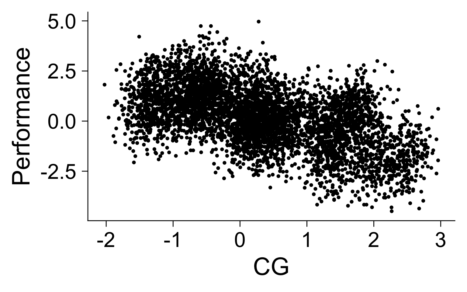
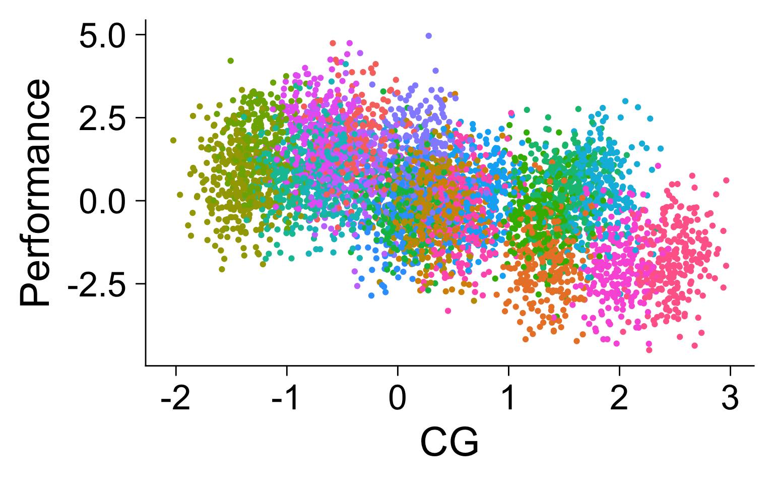
Fixed effects (for industry)
- Causal Diagram
- Simulation
- Regressions
- Simulation with correlated fixed effects
- Regressions with correlated fixed effects
Nind <- 20
N <- 5000
di <- tibble(
  ind_number = 1:Nind,
  ind_CG = rnorm(Nind, 0, 1),
  ind_performance = rnorm(Nind, 0, 1)
)
ds <- tibble(
    ind_number = sample(1:Nind, N, replace = TRUE)) %>%
  left_join(
    di, by = "ind_number") %>%
  mutate(
    CG = rnorm(N, .5 + ind_CG, .2),
    Performance = rnorm(N, 0 * CG + ind_performance, 1)
)| (1) | (2) | (3) | |
|---|---|---|---|
| * p < 0.1, ** p < 0.05, *** p < 0.01 | |||
| (Intercept) | -0.536*** | -0.709*** | |
| (0.021) | (0.119) | ||
| CG | 0.377*** | -0.019 | -0.019 |
| (0.018) | (0.070) | (0.079) | |
| factor(ind_number)2 | 0.626*** | ||
| (0.090) | |||
| factor(ind_number)3 | -0.923*** | ||
| (0.117) | |||
| factor(ind_number)4 | -0.200** | ||
| (0.092) | |||
| factor(ind_number)5 | -0.118 | ||
| (0.137) | |||
| factor(ind_number)6 | -1.163*** | ||
| (0.277) | |||
| factor(ind_number)7 | 0.353** | ||
| (0.172) | |||
| factor(ind_number)8 | -0.218 | ||
| (0.157) | |||
| factor(ind_number)9 | 1.484*** | ||
| (0.086) | |||
| factor(ind_number)10 | 1.708*** | ||
| (0.142) | |||
| factor(ind_number)11 | 0.909*** | ||
| (0.136) | |||
| factor(ind_number)12 | 0.815*** | ||
| (0.091) | |||
| factor(ind_number)13 | 0.868*** | ||
| (0.090) | |||
| factor(ind_number)14 | 2.120*** | ||
| (0.100) | |||
| factor(ind_number)15 | -2.404*** | ||
| (0.150) | |||
| factor(ind_number)16 | 2.314*** | ||
| (0.150) | |||
| factor(ind_number)17 | -1.187*** | ||
| (0.201) | |||
| factor(ind_number)18 | 0.315*** | ||
| (0.087) | |||
| factor(ind_number)19 | 0.161 | ||
| (0.189) | |||
| factor(ind_number)20 | -0.839*** | ||
| (0.229) | |||
| Num.Obs. | 5000 | 5000 | 5000 |
| R2 | 0.083 | 0.578 | 0.578 |
| R2 Within | 0.000 | ||
| Std.Errors | by: ind_number | ||
| FE: ind_number | X | ||
Nind <- 20
N <- 5000
correl <- -0.5
di <- tibble(
    ind_number = 1:Nind,
    ind_CG = rnorm(Nind, 0, 1)) %>%
  mutate(
    ind_performance = sqrt(1 - correl^2) * rnorm(Nind, 0, 1) + correl * ind_CG)
ds <- tibble(
    ind_number = sample(1:Nind, N, replace = TRUE)) %>%
  left_join(
    di, by = "ind_number") %>%
  mutate(
    CG = rnorm(N, .5 + ind_CG, .2),
    Performance = rnorm(N, 0 * CG + ind_performance, 1)
  )Nind <- 20
N <- 5000
correl <- -0.5
di <- tibble(
    ind_number = 1:Nind,
    ind_CG = rnorm(Nind, 0, 1)) %>%
  mutate(
    ind_performance = sqrt(1 - correl^2) * rnorm(Nind, 0, 1) + correl * ind_CG)
ds <- tibble(
    ind_number = sample(1:Nind, N, replace = TRUE)) %>%
  left_join(
    di, by = "ind_number") %>%
  mutate(
    CG = rnorm(N, .5 + ind_CG, .2),
    Performance = rnorm(N, 0 * CG + ind_performance, 1)
  )Nind <- 20
N <- 5000
correl <- -0.5
di <- tibble(
    ind_number = 1:Nind,
    ind_CG = rnorm(Nind, 0, 1)) %>%
  mutate(
    ind_performance = sqrt(1 - correl^2) * rnorm(Nind, 0, 1) + correl * ind_CG)
ds <- tibble(
    ind_number = sample(1:Nind, N, replace = TRUE)) %>%
  left_join(
    di, by = "ind_number") %>%
  mutate(
    CG = rnorm(N, .5 + ind_CG, .2),
    Performance = rnorm(N, 0 * CG + ind_performance, 1)
  )
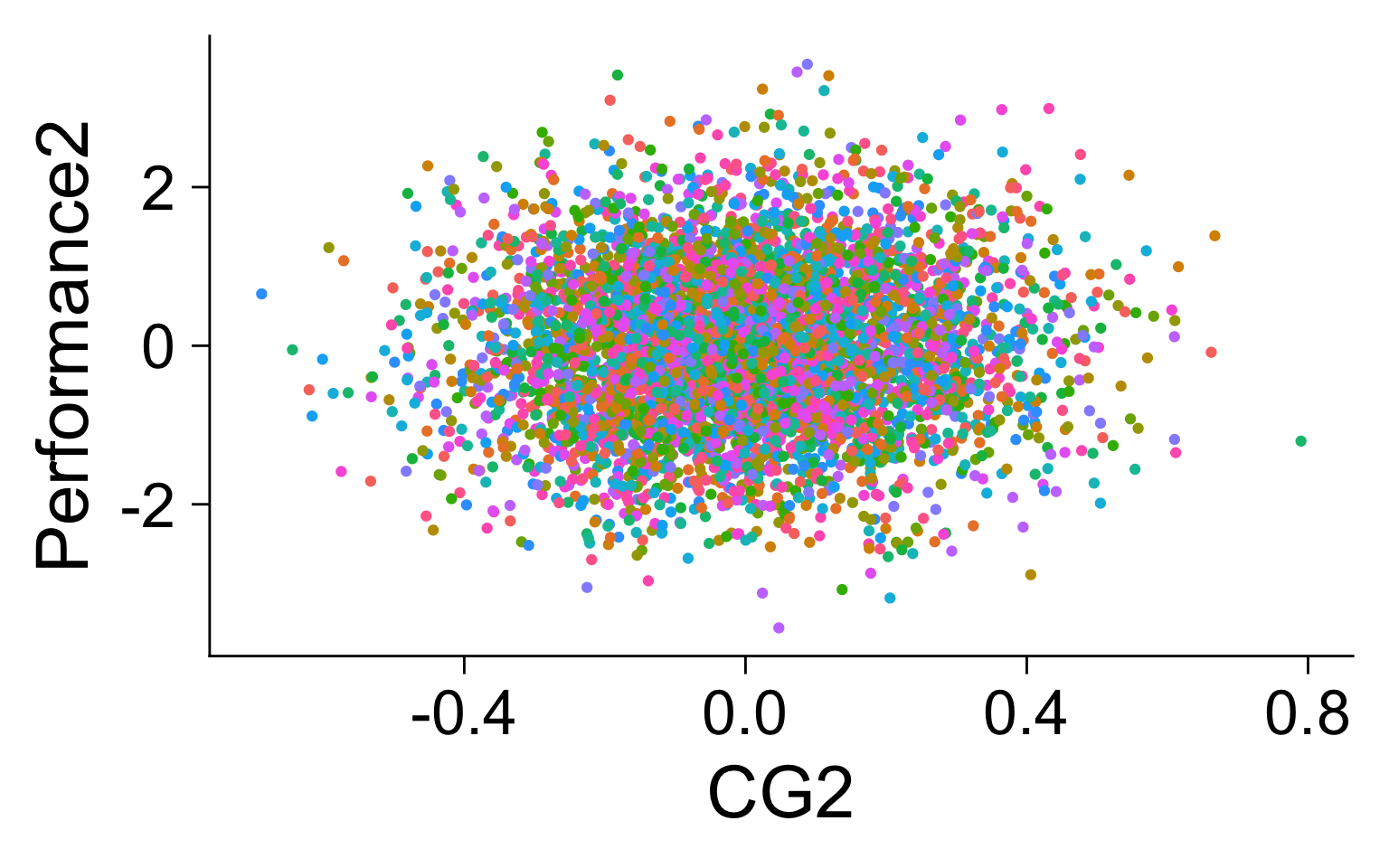
What do fixed effects do?
Speedboat Racing Example (Booth and Yamamura 2017)
- Mixed-sex and single-sex races determined by lottery (Randomisation)
- 7 race courses
- Multiple races in the same month and location
Results of Speedboat Races
Code
load(here("data", "booth_yamamura.Rdata"))
table <- as_tibble(table) %>%
  select(p_id, women_dat, time, ltime, mix_ra, course,
         race_id, yrmt_locid)
table_clean <- filter(table, complete.cases(table)) %>%
  select(ltime, women_dat, mix_ra, course, p_id, race_id,
         yrmt_locid)
ltime_reg <- feols(ltime ~ women_dat : mix_ra + mix_ra
                   | course + p_id + yrmt_locid,
                   cluster = "race_id",
                   data = table_clean)
msummary(ltime_reg, gof_omit = gof_omit, stars = stars)| (1) | |
|---|---|
| * p < 0.1, ** p < 0.05, *** p < 0.01 | |
| mix_ra | -0.002*** |
| (0.000) | |
| women_dat × mix_ra | 0.007*** |
| (0.001) | |
| Num.Obs. | 142346 |
| R2 | 0.361 |
| R2 Within | 0.001 |
| Std.Errors | by: race_id |
| FE: course | X |
| FE: p_id | X |
| FE: yrmt_locid | X |
Colliders and bad controls
Warning
Equilibrium models are very good at incorporating these effects!
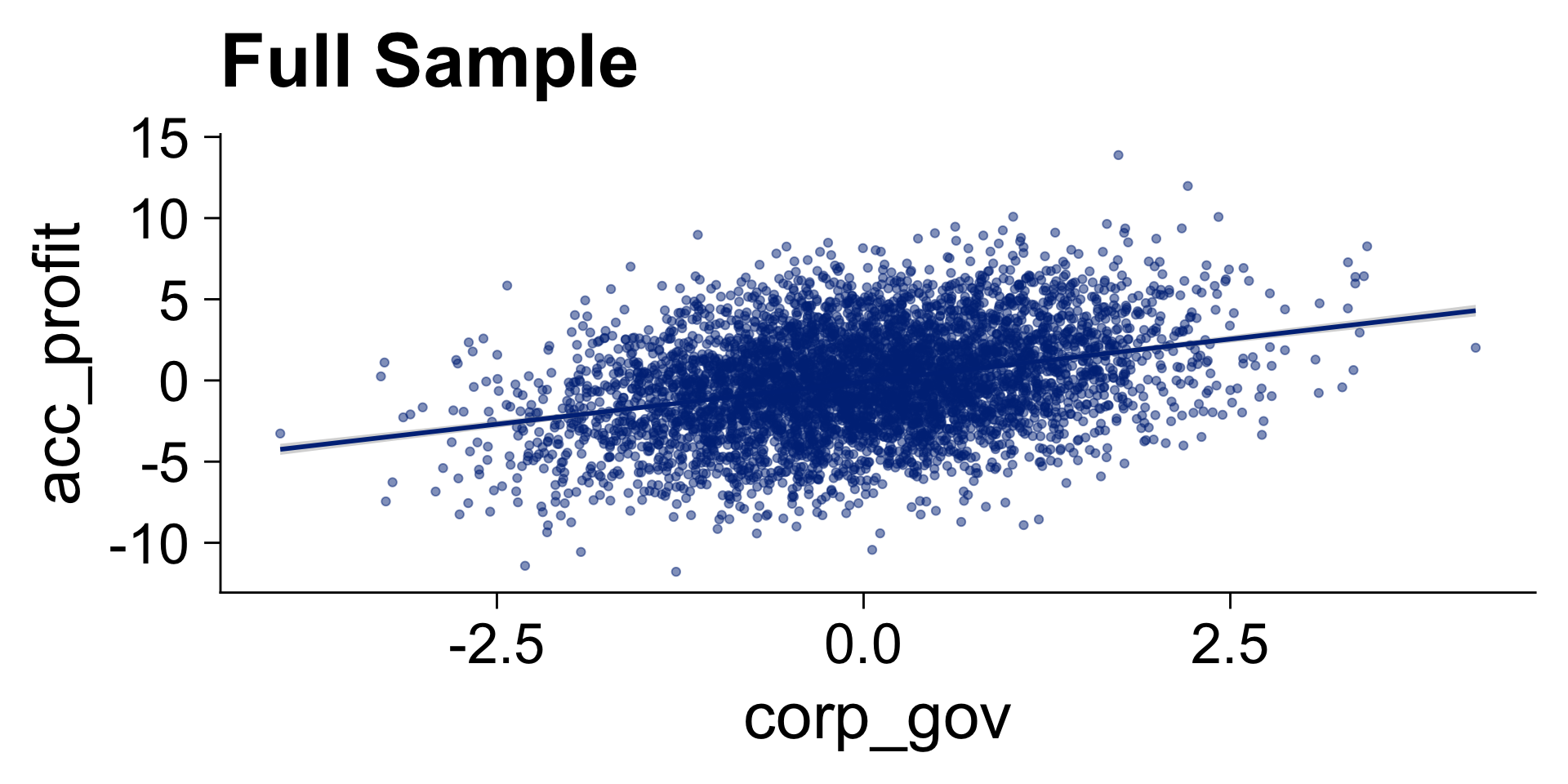
Bad Controls, Survival Bias, Selection Bias, Self-Selection Bias
Example in the assignment
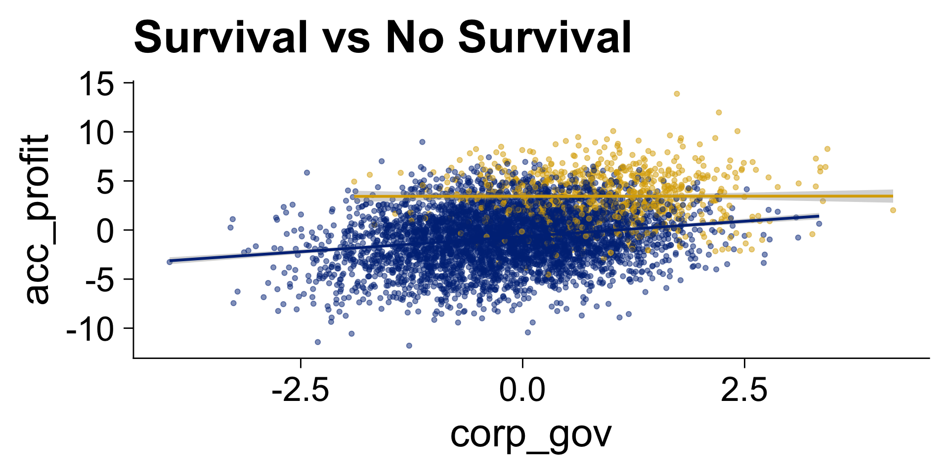
Simulation Bad Control
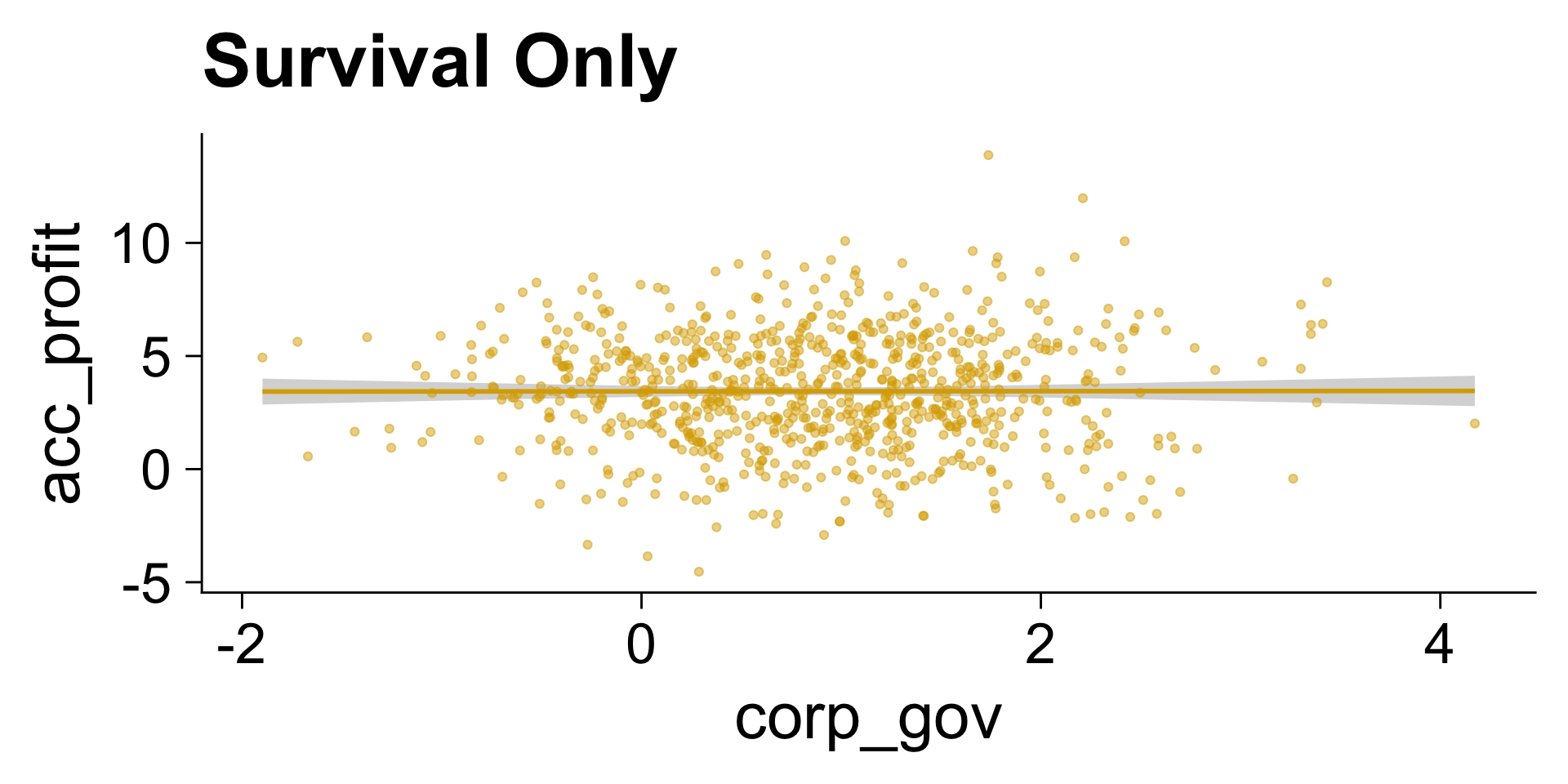
Survival Bias
lm1 <- lm(acc_profit ~ corp_gov, data = filter(d, survival == 1))
lm2 <- lm(acc_profit ~ corp_gov * survival, data = d)
msummary(list(lm1, lm2), gof_omit = gof_omit, stars = stars, output = "markdown")| (1) | (2) | |
|---|---|---|
| * p < 0.1, ** p < 0.05, *** p < 0.01 | ||
| (Intercept) | 3.437*** | -0.659*** |
| (0.125) | (0.043) | |
| corp_gov | 0.004 | 0.621*** |
| (0.100) | (0.045) | |
| survival | 4.096*** | |
| (0.142) | ||
| corp_gov × survival | -0.616*** | |
| (0.118) | ||
| Num.Obs. | 820 | 5000 |
| R2 | 0.000 | 0.266 |
Visualisation of Colliders (and Interactions)
Pitching Template
Pitching Format
- Description (Important)
- Title
- Research Question
- Key Paper
- Motivation
- THREE (IDioT) (Important)
- Idea
- Data
- Tools
Pitching Format
- Description (Important)
- Title
- Research Question
- Key Paper
- Motivation
- THREE (IDioT) (Important)
- Idea
- Data
- Tools
- TWO
- What’s new?
- So what?
- ONE contribution
- Other considerations.
References
Booth, Alison, and Eiji Yamamura. 2017. “Performance in Mixed-Sex and Single-Sex Competitions: What We Can Learn from Speedboat Races in Japan.” The Review of Economics and Statistics 100 (4): 581–93. https://doi.org/10.1162/rest_a_00715.
Huntington-Klein, Nick. 2021. The Effect: An Introduction to Research Design and Causality. First. Boca Raton: Chapman and Hall/CRC. https://doi.org/10.1201/9781003226055.
Control Variables Stijn Masschelein
