This is a non necessarily coherent collection of code that I used to develop my course material to teach the Baker, Larcker, and Wang (2022) paper on staggered difference-in-difference, specifically simulation 6. I used the opportunity to familiarise myself with some of the fastverse packages and I sprinkled some timing tests in the code here and there.1. If you are going to work with large datasets and just summarising the data takes a lot of computing time, switching over from the tidyverse to (some of) the fastverse packages might be a worthwhile investment of your time. My other interest in writing this all up is that it will allow me to test other estimators and other data generating processes.
R Setup
The here package helps with managing the different files associated with my teaching material. The tidyverse is what I normally use for data management and what I teach because I like the pedagogy but it’s not as fast compared to data.table and collapse. cowplot is my preference for decent default in plots. RPostgress is necessary to get the data from the WRDS server. fixest is the gold standard for regression estimators with fixed effects as of the time of writing. modelsummary is a package to create tables from regression objects. gof_omit and stars will override some of the defaults in modelsummary.run_wrds` is just a boolean to control whether I want to rerun the WRDS query.2
library(here)
here() starts at /Users/stijnmasschelein/Dropbox/github/site
── Conflicts ────────────────────────────────────────── tidyverse_conflicts() ──
✖ dplyr::filter() masks stats::filter()
✖ dplyr::lag()    masks stats::lag()
ℹ Use the conflicted package (<http://conflicted.r-lib.org/>) to force all conflicts to become errors
library(cowplot)
Attaching package: 'cowplot'

The following object is masked from 'package:lubridate':

    stamp
theme_set(theme_cowplot())library(collapse)
collapse 2.1.5, see ?`collapse-package` or ?`collapse-documentation`

Attaching package: 'collapse'

The following object is masked from 'package:tidyr':

    replace_na

The following object is masked from 'package:stats':

    D
library(data.table)
Attaching package: 'data.table'

The following object is masked from 'package:collapse':

    fdroplevels

The following objects are masked from 'package:lubridate':

    hour, isoweek, mday, minute, month, quarter, second, wday, week,
    yday, year

The following objects are masked from 'package:dplyr':

    between, first, last

The following object is masked from 'package:purrr':

    transpose
library(RPostgres)library(fixest)
Attaching package: 'fixest'

The following object is masked from 'package:collapse':

    fdim
The data comes from WRDS which has pretty good documentation on how to set up R and Rstudio to work. You do need an WRDS account though and they are not cheap. The code in this section does not run by default. 3.
I used Andrew Baker’s Github repository for the paper to replicate the underlying data but implement them in my own way. I don’t fully replicate the sample but it’s good enough for the example. I have slightly more observations and one day I will figure out where I went wrong.
sql1 <-"SELECT fyear, gvkey, oibdp, at, sich FROM COMP.FUNDA WHERE fyear > 1978 AND fyear < 2016 AND indfmt = 'INDL' AND datafmt = 'STD' AND popsrc = 'D' AND consol = 'C' AND fic = 'USA'"res <-dbSendQuery(wrds, sql1)dt <-as_tibble(dbFetch(res)) %>%rename_all(tolower)dbClearResult(res)roas <- dt %>%rename(year = fyear, firm = gvkey) %>%filter(!is.na(year), !is.na(at), !is.na(oibdp), at >0) %>%group_by(firm) %>%arrange(year) %>%mutate(roa = oibdp /lag(at)) %>%ungroup() %>%select(year, firm, roa, sich) %>%filter(!is.na(roa), year >1979)glimpse(roas)
# winsorize ROA at 99, and censor at -1wins <-function(x) {# winsorize and returncase_when(is.na(x) ~NA_real_, x <-1~-1, x >quantile(x, 0.99, na.rm =TRUE) ~quantile(x, 0.99, na.rm =TRUE),TRUE~ x )}# winsorize ROA by yearroas <- roas %>%group_by(year) %>%mutate(roa =wins(roa)) %>%arrange(firm, year) %>%ungroup()
The data was last modified on 2025-12-19 16:30:40.63027
Decomposition
If you are interested in creating you are own Baker file this is less relevant. It’s just my experimentation with the collapse package to mimic a naive calculation of year and time fixed effects with dplyr. Long story short, decomp_dplyr is almost 10 times slower than decomp_fast. With decent sized data and simulation exercises I am definitely more motivated to use the fastverse packages now. decomp_fixest is the correct decomposition in year and firm fixed effects. It’s not directly comparable to the other decompositions but given that it is actually the correct thing, it holds up pretty well in the timing.
Warning in microbenchmark::microbenchmark(dplyr = decomp_dplyr(), collapse =
decomp_fast(), : less accurate nanosecond times to avoid potential integer
overflows
Unit: milliseconds
     expr       min        lq      mean    median        uq       max neval
    dplyr 33.014553 34.856130 39.561814 37.013652 38.133669 99.135540    20
 collapse  1.641148  1.830896  2.272443  1.895389  2.139277  6.198052    20
   fixest 36.879295 39.413751 45.631204 41.339624 45.942407 98.203979    20
decomp <-decomp_fixest()glimpse(decomp)
List of 3
 $ ff   : Named num [1:12655] 0.0801 0.1526 -0.1387 0.2701 0.1107 ...
  ..- attr(*, "names")= chr [1:12655] "1003" "1004" "1007" "1009" ...
 $ fy   : Named num [1:36] 0.033907 0.028517 -0.002745 0 -0.000281 ...
  ..- attr(*, "names")= chr [1:36] "1980" "1981" "1982" "1983" ...
 $ resid: num [1:180397] 0.2995 0.0169 0.0626 0.1225 -0.0511 ...
Sampling
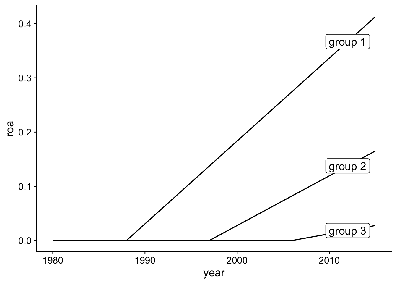
Now we can create new samples with the above derived fixed effects for the ROAs. I use the data.table package for most of the data manipulation. The first bit of code prepares everything that does not change across conditions in the observations data. We keep the identifier for the firm and year. The new firms data keeps the firm fixed effects the years data has the year firm fixed effects from the decomposition above. The residuals are stored as a vector and will represent the empirical distribution of the unexplaind part of the ROAs. The remaining variables reflect the treatment effects which are applied to three groups of states which are randomly assigned to one of the three groups 4
Warning: Removed 105 rows containing missing values or values outside the scale range
(`geom_label()`).
print(effect_plot)
Warning: Removed 105 rows containing missing values or values outside the scale range
(`geom_label()`).
The actual data simulation is in the new_sample function which again mostly uses data.table. The function goes through the following steps. I think I am adding more variation than the Baker et al. paper. So this is by no means a one-for-one replication but it allows me to build on extensions if I so want.
Each firm in the firm gets allocated a random firm fixed effect based on the empirical distribution of the firm fixed effects and gets allocated to one of 50 states.
Based on the state, I assign the firm to a treatment group and treatment effect.
Each year gets a randomly sampled year fixed effect based on the empirical distribution.
The two fixed effects are merged to the firm-year observations.
The simulated ROA is calculated based on the fixed effects, the treatment effect, and random residuals.
During the development of the function I kept track of the timing of the function. Overall, I am quite impressed how fast this was.
Unit: milliseconds
   expr      min       lq     mean   median       uq     max neval
 sample 14.45795 17.47049 23.27825 19.10744 21.25053 90.0704   100
Analyse
For now I focus on three estimators. The traditional two-way fixed effect estimator, the Sun and Abraham (2021) estimator, and the Callaway and Sant’Anna (2021) estimator. The Sun and Abraham (2021) estimator is easy to implement as a fixed effect regression and conceptually easy to explain because the hard work is done by only using the appropriate data which allows for the appropriate comparison. The Callaway and Sant’Anna (2021) is more robust has and is easier to extend to include selection effects, automatic selection of control groups, and additional control variables.
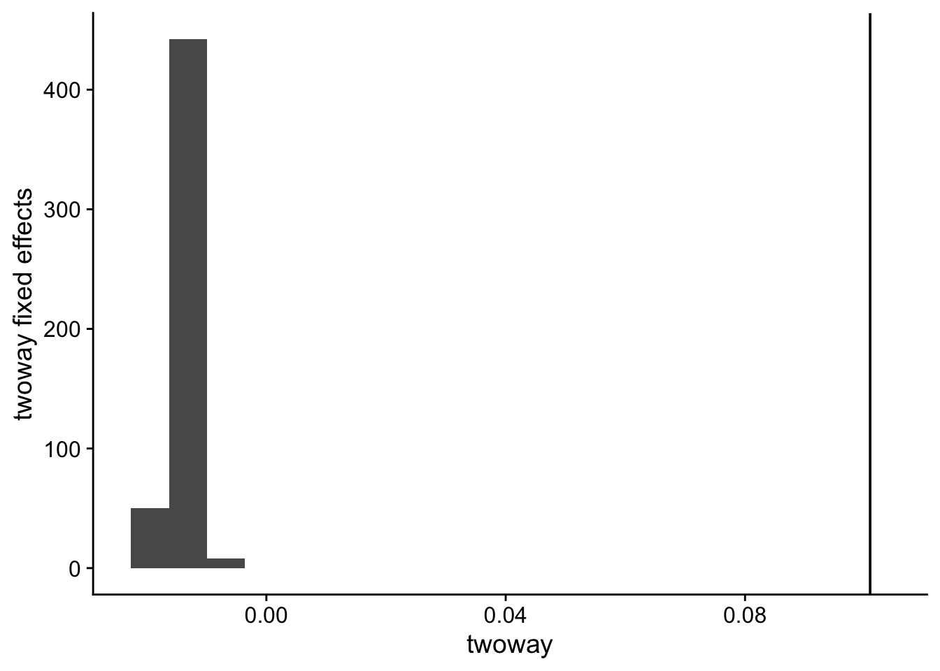
Two-way Fixed Effects
new <-new_sample()twoway <-feols(roa ~ifelse(year >= treatment_group, 1, 0)| year + firm,cluster ="state", data = new)etable(twoway)
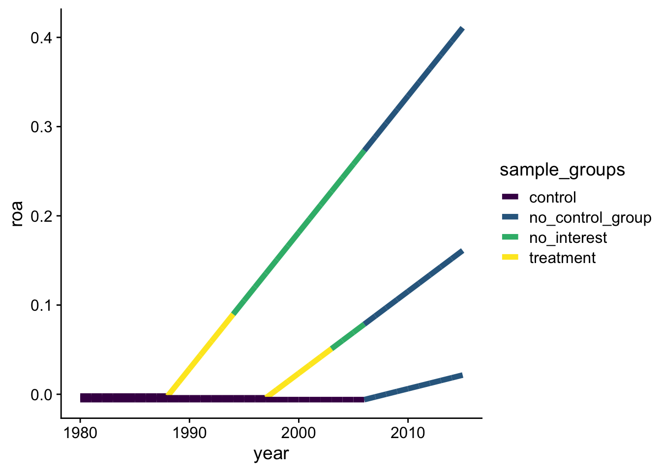
The hard work is done by making sure that we make no invalid comparisons. I try to explain this with the following figure. I assume we are only interested in the treatment effect 5 years after the implementation of the treatment. For group 3 who gets the treatment last, there is not appropriate control group (no_control_group) so we do not use this group after the treatment. For the other groups, we delete the data more than 5 years after treatment (no_interest). We are left with controls which are all pre treatment (control) and the 5 years of treatment in group 1 and 2 (treatment).
plot_dt[, `:=`(roa = roa -0.002* group,sample_groups =case_when( year >=2007-1~"no_control_group", year - treatment_groups[group] >5-1~"no_interest", year < treatment_groups[group] -1~"control", year >= treatment_groups[group] -1~"treatment" ))]sun_plot <-ggplot(plot_dt, aes(y = roa, x = year, group = group,label = label, colour = sample_groups)) +geom_line(size =2) + viridis::scale_colour_viridis(discrete = T)
Warning: Using `size` aesthetic for lines was deprecated in ggplot2 3.4.0.
ℹ Please use `linewidth` instead.
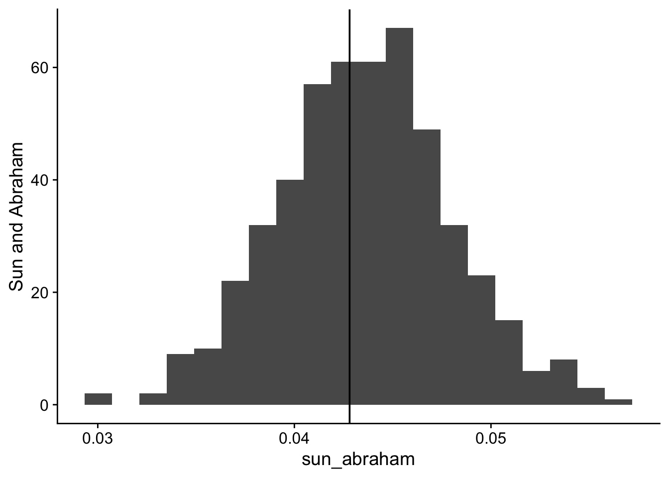
The actual code to run the Sun and Abraham (2021) estimator is available in fixest. We first need to construct the cleaned data set following the figure above. Next, we run the regression with fixest and use the sunab function, which automatically creates indicators for each relative year - treatment group combination. It excludes rel_year = -1 which is the year before the treatment and the benchmark to which all the estimated coefficients can be compared.
The default output for the Sun and Abraham estimator is to report the aggregated5 relative time coefficients. The overall average treatment effect can be extracted with the summary function.
For the Callaway and Sant’Anna code to work we first need to set the treatment group variable to 0 for the group that is never treated (in the subsample). And the code needs to exclude all firms that don’t have any pre-treatment observations.
Warning in did_standarization(data, args): 8987 units are missing in some
periods. Converting to balanced panel by dropping them.
ATT_cs <-aggte(cs, type ="simple")ATT_cs$overall.att
[1] 0.09987021
True ATT
The true ATT will be different if we use the full sample or restrict the treated observations to 5 years after the treatment for group 1 and 2 or any other exlusion. The following code calculates the expected true ATT for the full sample or by cohort. The true_att calculation exploits the linear increase in the treatment effect.
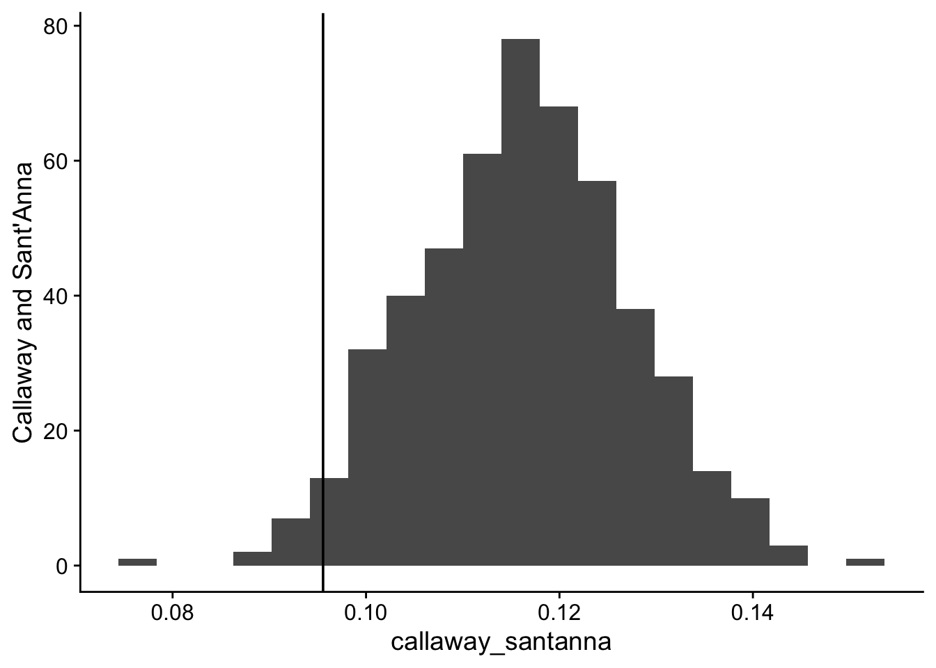
Everything is now in place to run a simulation that simulates new data and runs the two-way fixed effect OLS estimator, the Sun and Abraham (2021) estimator and the Callaway and Sant’Anna (2021) estimator. I extract the estimate of the ATT from both and save them as the results.
The rest of the code runs the simulation nsim times and plots the estimate with the expected true ATT.
     twoway           sun_abraham      callaway_santanna
 Min.   :-0.019456   Min.   :0.03004   Min.   :0.0764
 1st Qu.:-0.014987   1st Qu.:0.04075   1st Qu.:0.1090
 Median :-0.013805   Median :0.04365   Median :0.1166
 Mean   :-0.013747   Mean   :0.04359   Mean   :0.1164
 3rd Qu.:-0.012435   3rd Qu.:0.04654   3rd Qu.:0.1238
 Max.   :-0.006342   Max.   :0.05650   Max.   :0.1517
Baker, Andrew C., David F. Larcker, and Charles C. Y. Wang. 2022. “How Much Should We Trust Staggered Difference-in-Differences Estimates?”Journal of Financial Economics 144 (2): 370–95. https://doi.org/10.1016/j.jfineco.2022.01.004.
Callaway, Brantly, and Pedro H. C. Sant’Anna. 2021. “Difference-in-Differences with Multiple Time Periods.”Journal of Econometrics, Themed Issue: Treatment Effect 1, 225 (2): 200–230. https://doi.org/10.1016/j.jeconom.2020.12.001.
Sun, Liyang, and Sarah Abraham. 2021. “Estimating Dynamic Treatment Effects in Event Studies with Heterogeneous Treatment Effects.”Journal of Econometrics, Themed Issue: Treatment Effect 1, 225 (2): 175–99. https://doi.org/10.1016/j.jeconom.2020.09.006.
Footnotes
You may or may not be interested in this but there you go. It’s free.↩︎
This is slightly different than in the Baker et al. paper. I allow that by random chance some of the groups are larger than the other while the Baker et al. simulation keeps the groups (almost) equal in size. I was too lazy to change it when I noticed the difference but I am also interested in what happens to the average treatment effect if some group effects are estimated more precisely so my simulation is at least consistent with that goal↩︎