Rows: 130,358
Columns: 26
$ ticker <chr> "A2", "A2", "A2", "A2", "A2", "A2", "A2", "AA0A", "AA0A",…
$ actual <dbl> -0.0400, -0.1100, -0.1100, -0.0500, -0.0700, -0.1000, -0.…
$ pdf <chr> "D", "D", "D", "D", "D", "D", "D", "D", "D", "D", "D", "D…
$ anndats_act <date> 2004-10-21, 2005-01-26, 2005-04-27, 2005-07-27, 2005-10-…
$ gvkey <chr> "001081", "001081", "001081", "001081", "001081", "001081…
$ permno <dbl> 10560, 10560, 10560, 10560, 10560, 10560, 10560, 10656, 1…
$ cusip <chr> "00392410", "00392410", "00392410", "00392410", "00392410…
$ rdq <date> 2004-10-21, 2005-01-26, 2005-04-27, 2005-07-27, 2005-10-…
$ anndat <date> 2004-10-21, 2005-01-26, 2005-04-27, 2005-07-27, 2005-10-…
$ N <int> 1, 2, 3, 2, 4, 5, 4, 1, 1, 1, 1, 1, 1, 2, 2, 1, 1, 3, 2, …
$ median <dbl> -0.09000, -0.08965, -0.05740, -0.03700, -0.10610, -0.0783…
$ mean <dbl> -0.0900000, -0.0896500, -0.0680000, -0.0370000, -0.100550…
$ mean_days <dbl> 21.000000, 8.000000, 6.666667, 13.500000, 7.000000, 9.200…
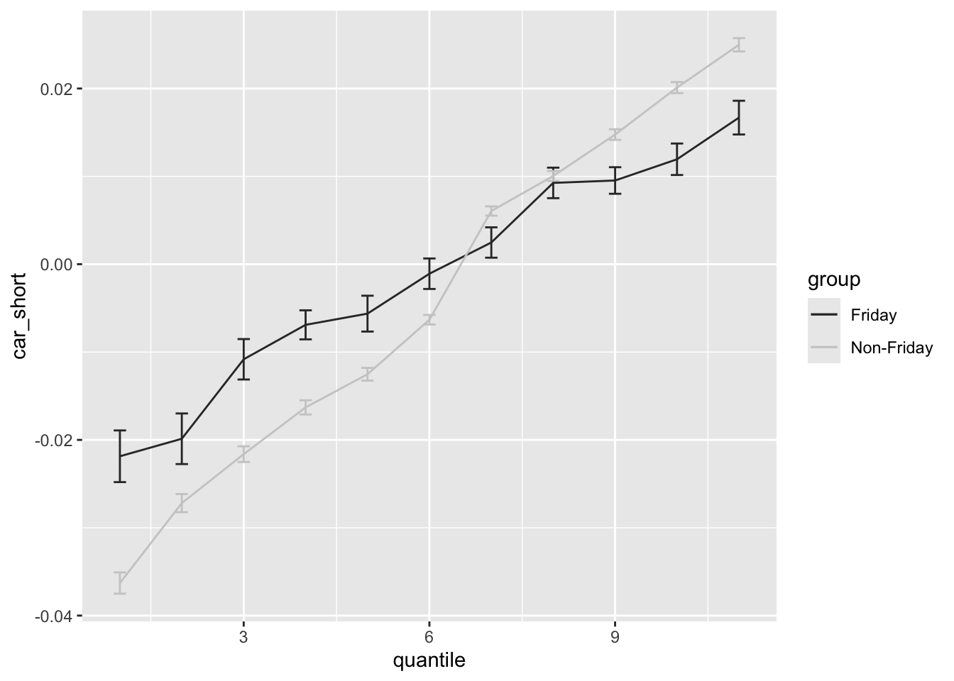
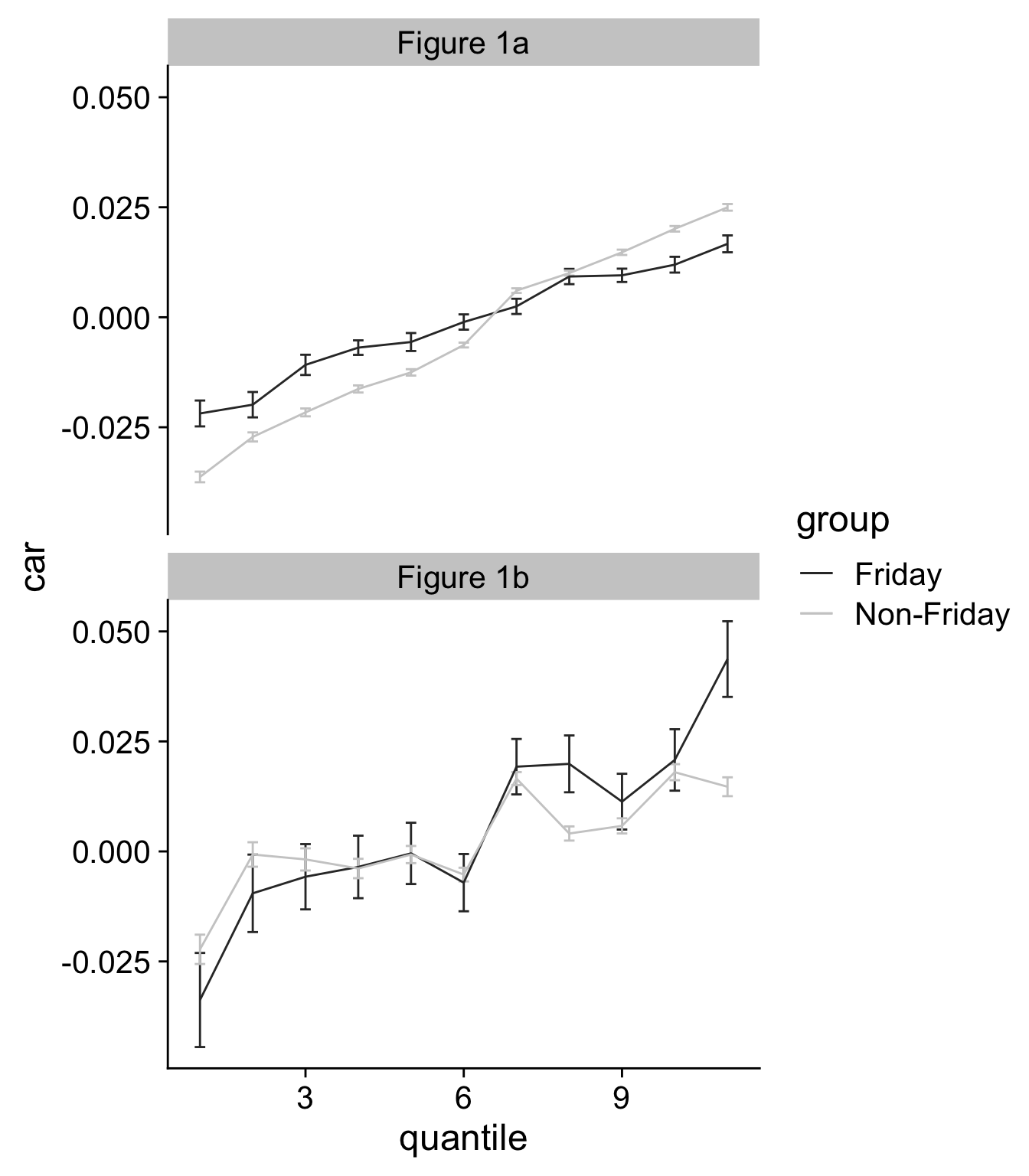
$ car_short <dbl> 0.097290562, 0.036462040, -0.063605028, -0.004177245, -0.…
$ car_long <dbl> 0.01028628, -0.20959780, 0.05661647, -0.18368201, 0.20741…
$ date_minus5 <date> 2004-10-16, 2005-01-21, 2005-04-22, 2005-07-22, 2005-10-…
$ date <date> 2004-10-15, 2005-01-21, 2005-04-22, 2005-07-22, 2005-10-…
$ prc <dbl> 5.63, 5.89, 4.53, 5.00, 3.26, 4.02, 4.28, 16.75, 15.66, 1…
$ market_value <dbl> 2478185.2, 2592630.8, 1993992.8, 2200875.0, 1434970.5, 17…
$ surprise <dbl> 0.0088809947, -0.0034550085, -0.0116114790, -0.0026000000…
$ weekday <ord> Thu, Wed, Wed, Wed, Wed, Wed, Wed, Thu, Thu, Wed, Thu, Th…
$ group <chr> "Non-Friday", "Non-Friday", "Non-Friday", "Non-Friday", "…
$ year <dbl> 2004, 2005, 2005, 2005, 2005, 2006, 2006, 2003, 2003, 200…
$ sign <chr> "positive", "negative", "negative", "negative", "positive…
$ quintile <int> 5, 2, 1, 3, 5, 2, 3, 3, 3, 4, 2, 1, 3, 2, 5, 2, 4, 5, 5, …
$ quantile <dbl> 11, 2, 1, 3, 11, 2, 3, 9, 9, 4, 2, 6, 9, 2, 11, 2, 10, 11…